
도찐개찐
[데이터분석] 13. 다중회귀분석 본문
import numpy as np
import pandas as pd
import matplotlib.pyplot as plt
import matplotlib as mpl
import seaborn as sns
from sklearn.datasets import load_boston
from sklearn.datasets import fetch_california_housing
from statsmodels.formula.api import ols
fontpath = '/home/bigdata/py39/lib/python3.9/site-packages/matplotlib/mpl-data/fonts/ttf/NanumGothic.ttf'
fname = mpl.font_manager.FontProperties(fname=fontpath).get_name()
mpl.rcParams['font.family'] = 'NanumGothic'
mpl.rcParams['font.size'] = 12
mpl.rcParams['axes.unicode_minus'] = False다중회귀분석
- 단일 회귀분석에 비해 변수가 2개이상 증가
- 기술통계학이나 추론통계학 상의 주요 기법
- 종속변수 $y$를 보다 더 잘 설명하고 예측하기 위해 여러 독립변수 $x$를 사용함
- 다중회귀방정식 :
$ \hat y = a + bx_1 + cx_2 + dx_3 + .... $ - 하지만, 독립변수가 3개 이상인 경우 그래프로 표현하기 어려워지므로
- 보통 $ \hat y = a + bx_1 + cx_2 $ 정도로만 고려하는 것이 좋음
부동산회사 난방비 예측 모델 생성
houses = pd.read_csv('https://raw.githubusercontent.com/siestageek/datasets/master/txt/houses.txt',
                     sep='\t', encoding='CP949')
houses.info()
<class 'pandas.core.frame.DataFrame'>
RangeIndex: 20 entries, 0 to 19
Data columns (total 4 columns):
# Column Non-Null Count Dtype
--- ------ -------------- -----
0 난방비 20 non-null int64
1 평균외부기온 20 non-null int64
2 단열재 20 non-null int64
3 난방사용연수 20 non-null int64
dtypes: int64(4)
memory usage: 768.0 byteshouses.corr()| 난방비 | 평균외부기온 | 단열재 | 난방사용연수 | |
|---|---|---|---|---|
| 난방비 | 1.000000 | -0.811509 | -0.257101 | 0.536728 |
| 평균외부기온 | -0.811509 | 1.000000 | -0.103016 | -0.485988 |
| 단열재 | -0.257101 | -0.103016 | 1.000000 | 0.063617 |
| 난방사용연수 | 0.536728 | -0.485988 | 0.063617 | 1.000000 |
sns.heatmap(houses.corr(), annot=True, fmt='.2f')<AxesSubplot:>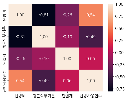
sns.pairplot(houses, diag_kind='kde')<seaborn.axisgrid.PairGrid at 0x7f6562a9aee0>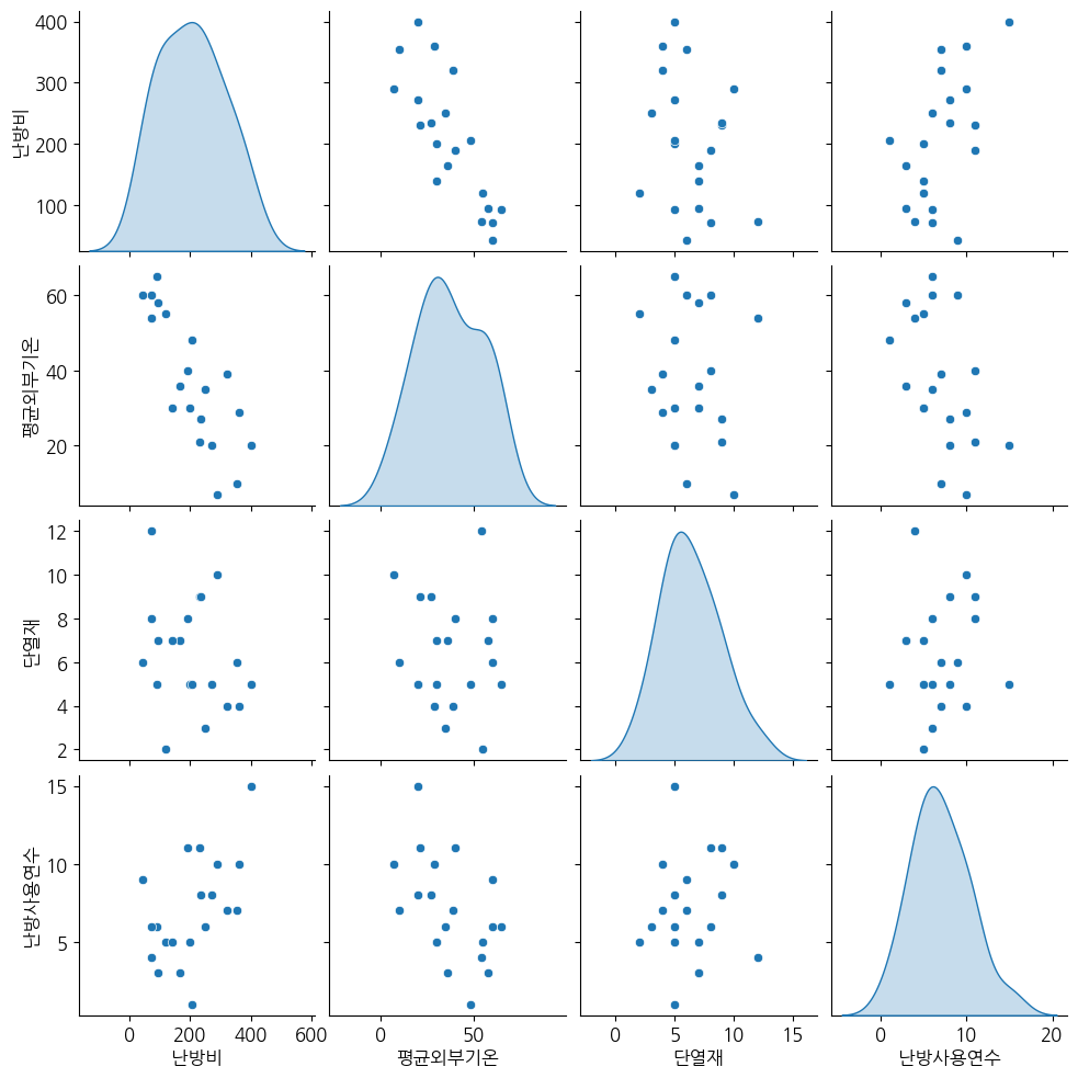
avg = houses.iloc[:, 1]
nan = houses.iloc[:, 0]
a_mean = np.mean(avg)
n_mean = np.mean(nan)
plt.scatter(nan, avg, color='red')
plt.axvline(n_mean)
plt.axhline(a_mean)<matplotlib.lines.Line2D at 0x7f655facaee0>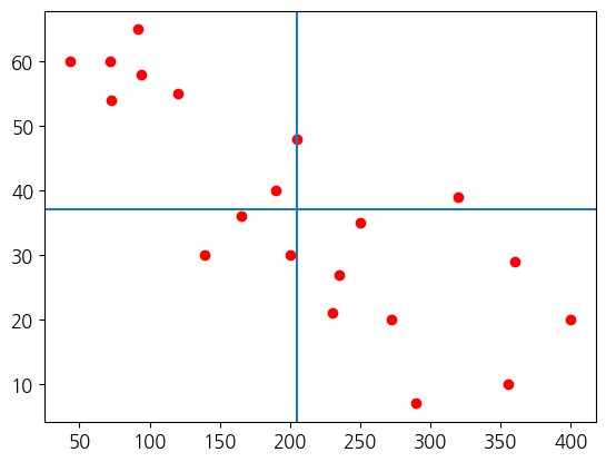
np.cov(nan, avg)[0, 1]-1495.6315789473683np.corrcoef(nan, avg)[0, 1]-0.8115088354934337다중회귀모형 분석방법
- 수정된 결정계수
- 독립변수의 수가 증가할수록 예측력이 좋아져서
- 결정계수의 수치가 증가하는 경향이 있음
- 이러한 효과를 상쇄시킨 수정된 결정계수를 사용
- 모든 회귀계수들의 유의성을 판단 : $F$분포
- 다중회귀계수가 모두 0인지 검정함
- 귀무가설 : 각 계수 $a$,$b$,$c$ 가 0이다
- 대립가설 : 각 계수 $a$,$b$,$c$ 가 0이 아니다
- 유의수준 0.05로 정함, 양측검정
- 개별회귀계수에 대한 평가 : $t$분포
- 귀무가설 : 계수 $x$ 가 0이다
- 대립가설 : 계수 $x$ 가 0이 아니다
- 유의수준 0.05로 정함, 양측검정
부동산회사 난방비 다중 회귀분석
부동산회사 난방비 다중 회귀분석
# 분석 대상컬럼은 '종속변수~독립변수1+독립변수2' 형태의 식으로 작성해야 함.
# 간단하게 '종속변수~.' 으로도 사용
model = ols('난방비~평균외부기온+단열재+난방사용연수', data=houses).fit()
# model = ols('난방비~.', data=houses).fit()
print(model.summary())
OLS Regression Results
==============================================================================
Dep. Variable: 난방비 R-squared: 0.804
Model: OLS Adj. R-squared: 0.767
Method: Least Squares F-statistic: 21.90
Date: Mon, 14 Nov 2022 Prob (F-statistic): 6.56e-06
Time: 01:17:16 Log-Likelihood: -104.80
No. Observations: 20 AIC: 217.6
Df Residuals: 16 BIC: 221.6
Df Model: 3
Covariance Type: nonrobust
==============================================================================
coef std err t P>|t| [0.025 0.975]
------------------------------------------------------------------------------
Intercept 427.1938 59.601 7.168 0.000 300.844 553.543
평균외부기온 -4.5827 0.772 -5.934 0.000 -6.220 -2.945
단열재 -14.8309 4.754 -3.119 0.007 -24.910 -4.752
난방사용연수 6.1010 4.012 1.521 0.148 -2.404 14.606
==============================================================================
Omnibus: 0.464 Durbin-Watson: 1.538
Prob(Omnibus): 0.793 Jarque-Bera (JB): 0.558
Skew: 0.100 Prob(JB): 0.757
Kurtosis: 2.207 Cond. No. 218.
==============================================================================
Notes:
[1] Standard Errors assume that the covariance matrix of the errors is correctly specified.# 회귀식 : y = -4.58평균외부기온 단열재 -14.83단열재 + 6.1난방사용변수 + 427.19 (요약 coef 기준 계산)난방사용연수를 제외하고 회귀모델 재생성
# 분석 대상컬럼은 '종속변수~독립변수1+독립변수2' 형태의 식으로 작성해야 함.
# 간단하게 '종속변수~.' 으로도 사용
model = ols('난방비~평균외부기온+단열재', data=houses).fit()
# model = ols('난방비~.', data=houses).fit()
print(model.summary())
OLS Regression Results
==============================================================================
Dep. Variable: 난방비 R-squared: 0.776
Model: OLS Adj. R-squared: 0.749
Method: Least Squares F-statistic: 29.42
Date: Mon, 14 Nov 2022 Prob (F-statistic): 3.01e-06
Time: 01:17:16 Log-Likelihood: -106.15
No. Observations: 20 AIC: 218.3
Df Residuals: 17 BIC: 221.3
Df Model: 2
Covariance Type: nonrobust
==============================================================================
coef std err t P>|t| [0.025 0.975]
------------------------------------------------------------------------------
Intercept 490.2859 44.410 11.040 0.000 396.589 583.983
평균외부기온 -5.1499 0.702 -7.337 0.000 -6.631 -3.669
단열재 -14.7181 4.934 -2.983 0.008 -25.128 -4.308
==============================================================================
Omnibus: 0.228 Durbin-Watson: 1.524
Prob(Omnibus): 0.892 Jarque-Bera (JB): 0.398
Skew: 0.183 Prob(JB): 0.820
Kurtosis: 2.415 Cond. No. 155.
==============================================================================
Notes:
[1] Standard Errors assume that the covariance matrix of the errors is correctly specified.
다중회귀모델 해석
- $회귀식 : y = -5.14평균외부기온 -14.71단열재 + 490.28$ (요약 coef 기준 계산)
- 1) 평균외부기온 1도 증가 => 난방비는 5.4 감소
- 2) 단열재 두께가 1cm 증가 => 난방비는 -14.71 감소
- 3) 난방기연수가 1년증가 => 난방비는 6.10 증가
- 4) 주택 자체 기본 난방비 => 난방비는 427
다중회귀분석
- 단일 회귀분석에 비해 변수가 2개이상 증가
- 기술통계학이나 추론통계학 상의 주요 기법
- 종속변수 $y$를 보다 더 잘 설명하고 예측하기 위해 여러 독립변수 $x$를 사용함
- 다중회귀방정식 :
$ \hat y = a + bx_1 + cx_2 + dx_3 + .... $ - 하지만, 독립변수가 3개 이상인 경우 그래프로 표현하기 어려워지므로
- 보통 $ \hat y = a + bx_1 + cx_2 $ 정도로만 고려하는 것이 좋음# 다중회귀모형 분석방법
- 수정된 결정계수
- 독립변수의 수가 증가할수록 예측력이 좋아져서
- 결정계수의 수치가 증가하는 경향이 있음
- 이러한 효과를 상쇄시킨 수정된 결정계수를 사용
- 모든 회귀계수들의 유의성을 판단 : $F$분포
- 다중회귀계수가 모두 0인지 검정함
- 귀무가설 : 각 계수 $a$,$b$,$c$ 가 0이다
- 대립가설 : 각 계수 $a$,$b$,$c$ 가 0이 아니다
- 유의수준 0.05로 정함, 양측검정
- 개별회귀계수에 대한 평가 : $t$분포
- 귀무가설 : 계수 $x$ 가 0이다
- 대립가설 : 계수 $x$ 가 0이 아니다
- 유의수준 0.05로 정함, 양측검정
독립변수 최적화
- 독립변수가 많을때 유의한 계수를 포함시키고 유의하지 않은 계수를 제외시켜 구한 회귀방정식은 간단해지고 이해하기 쉬워짐
- 가능하다면 적은수의 독립변수를 포함하는 것이 좋음
- 다중회귀식에 포함할 수 있는 독립변수들을 효과적으로 선별할 수 있는 분석방법
- 단계적 회귀법, 단계적 변수선택법
독립변수 소거법
- 전진소거법 : 변수를 하나씩 추가함 => 중요도가 높은 변수부터 추가
- 후진소거법 : 모든 변수를 추가해둔 상태에서 $p$값이 높은 변수부터 제거
- 단계적 선택법 : 전진/후진 소거법을 적절히 조합
- 변수소거시 참고해야하는 지표 : AIC, BIC
- 모델에 $k$개의 변수를 추가하면 $2k$만큼 불이익이 추가함
- 따라서, 변수 소거시 AIC, BIC가 낮아지는 모델을 찾으면 됨
변수소거(후진소거)를 이용한 부동산회사 난방비 다중회귀 분석
# 후진소거 1
model = ols('난방비~평균외부기온+단열재+난방사용연수', data=houses).fit()
print(model.summary())

# 수정 된 결정계수 0.767
# AIC : 217
# => 난방사용연수 계수가 유의하지 않음(0.148) - 제거
OLS Regression Results
==============================================================================
Dep. Variable: 난방비 R-squared: 0.804
Model: OLS Adj. R-squared: 0.767
Method: Least Squares F-statistic: 21.90
Date: Mon, 14 Nov 2022 Prob (F-statistic): 6.56e-06
Time: 01:17:16 Log-Likelihood: -104.80
No. Observations: 20 AIC: 217.6
Df Residuals: 16 BIC: 221.6
Df Model: 3
Covariance Type: nonrobust
==============================================================================
coef std err t P>|t| [0.025 0.975]
------------------------------------------------------------------------------
Intercept 427.1938 59.601 7.168 0.000 300.844 553.543
평균외부기온 -4.5827 0.772 -5.934 0.000 -6.220 -2.945
단열재 -14.8309 4.754 -3.119 0.007 -24.910 -4.752
난방사용연수 6.1010 4.012 1.521 0.148 -2.404 14.606
==============================================================================
Omnibus: 0.464 Durbin-Watson: 1.538
Prob(Omnibus): 0.793 Jarque-Bera (JB): 0.558
Skew: 0.100 Prob(JB): 0.757
Kurtosis: 2.207 Cond. No. 218.
==============================================================================
Notes:
[1] Standard Errors assume that the covariance matrix of the errors is correctly specified.# 후진소거 2
model = ols('난방비~평균외부기온+단열재', data=houses).fit()
print(model.summary())
# 수정 된 결정계수 0.767 > 0.749
# AIC : 217.6 > 218.3
# => 난방사용연수 계수가 유의하지 않음(0.148) - 제거 OLS Regression Results
==============================================================================
Dep. Variable: 난방비 R-squared: 0.776
Model: OLS Adj. R-squared: 0.749
Method: Least Squares F-statistic: 29.42
Date: Mon, 14 Nov 2022 Prob (F-statistic): 3.01e-06
Time: 01:17:16 Log-Likelihood: -106.15
No. Observations: 20 AIC: 218.3
Df Residuals: 17 BIC: 221.3
Df Model: 2
Covariance Type: nonrobust
==============================================================================
coef std err t P>|t| [0.025 0.975]
------------------------------------------------------------------------------
Intercept 490.2859 44.410 11.040 0.000 396.589 583.983
평균외부기온 -5.1499 0.702 -7.337 0.000 -6.631 -3.669
단열재 -14.7181 4.934 -2.983 0.008 -25.128 -4.308
==============================================================================
Omnibus: 0.228 Durbin-Watson: 1.524
Prob(Omnibus): 0.892 Jarque-Bera (JB): 0.398
Skew: 0.183 Prob(JB): 0.820
Kurtosis: 2.415 Cond. No. 155.
==============================================================================
Notes:
[1] Standard Errors assume that the covariance matrix of the errors is correctly specified.변수소거(전진소거)를 이용한 부동산회사 난방비 다중회귀 분석
# 전진소거 1
model = ols('난방비 ~ 평균외부기온', data=houses).fit()
print(model.summary())

# 수정된 결정계수 : 0.408
# AIC : 264.7
OLS Regression Results
==============================================================================
Dep. Variable: 난방비 R-squared: 0.659
Model: OLS Adj. R-squared: 0.640
Method: Least Squares F-statistic: 34.72
Date: Mon, 14 Nov 2022 Prob (F-statistic): 1.41e-05
Time: 01:17:16 Log-Likelihood: -110.36
No. Observations: 20 AIC: 224.7
Df Residuals: 18 BIC: 226.7
Df Model: 1
Covariance Type: nonrobust
==============================================================================
coef std err t P>|t| [0.025 0.975]
------------------------------------------------------------------------------
Intercept 388.8020 34.241 11.355 0.000 316.865 460.739
평균외부기온 -4.9342 0.837 -5.892 0.000 -6.694 -3.175
==============================================================================
Omnibus: 2.208 Durbin-Watson: 1.367
Prob(Omnibus): 0.332 Jarque-Bera (JB): 1.630
Skew: 0.683 Prob(JB): 0.443
Kurtosis: 2.698 Cond. No. 98.6
==============================================================================
Notes:
[1] Standard Errors assume that the covariance matrix of the errors is correctly specified.# 전진소거 2
model = ols('난방비 ~ 평균외부기온 + 단열재', data=houses).fit()
print(model.summary())
# 수정된 결정계수 : 0.408 > 0.590
# AIC : 258.3 OLS Regression Results
==============================================================================
Dep. Variable: 난방비 R-squared: 0.776
Model: OLS Adj. R-squared: 0.749
Method: Least Squares F-statistic: 29.42
Date: Mon, 14 Nov 2022 Prob (F-statistic): 3.01e-06
Time: 01:17:16 Log-Likelihood: -106.15
No. Observations: 20 AIC: 218.3
Df Residuals: 17 BIC: 221.3
Df Model: 2
Covariance Type: nonrobust
==============================================================================
coef std err t P>|t| [0.025 0.975]
------------------------------------------------------------------------------
Intercept 490.2859 44.410 11.040 0.000 396.589 583.983
평균외부기온 -5.1499 0.702 -7.337 0.000 -6.631 -3.669
단열재 -14.7181 4.934 -2.983 0.008 -25.128 -4.308
==============================================================================
Omnibus: 0.228 Durbin-Watson: 1.524
Prob(Omnibus): 0.892 Jarque-Bera (JB): 0.398
Skew: 0.183 Prob(JB): 0.820
Kurtosis: 2.415 Cond. No. 155.
==============================================================================
Notes:
[1] Standard Errors assume that the covariance matrix of the errors is correctly specified.# 전진소거 3
model = ols('난방비 ~ 평균외부기온 + 난방사용연수', data=houses).fit()
print(model.summary())
# 수정된 결정계수 : 0.408 > 0.648
# AIC : 225.1
# 단, 평균외부기온 유의확률이 크므로 의미 없음 OLS Regression Results
==============================================================================
Dep. Variable: 난방비 R-squared: 0.685
Model: OLS Adj. R-squared: 0.648
Method: Least Squares F-statistic: 18.49
Date: Mon, 14 Nov 2022 Prob (F-statistic): 5.43e-05
Time: 01:17:16 Log-Likelihood: -109.55
No. Observations: 20 AIC: 225.1
Df Residuals: 17 BIC: 228.1
Df Model: 2
Covariance Type: nonrobust
==============================================================================
coef std err t P>|t| [0.025 0.975]
------------------------------------------------------------------------------
Intercept 326.9753 61.761 5.294 0.000 196.671 457.279
평균외부기온 -4.3835 0.947 -4.629 0.000 -6.381 -2.386
난방사용연수 5.9059 4.935 1.197 0.248 -4.507 16.319
==============================================================================
Omnibus: 1.478 Durbin-Watson: 1.445
Prob(Omnibus): 0.478 Jarque-Bera (JB): 1.281
Skew: 0.542 Prob(JB): 0.527
Kurtosis: 2.400 Cond. No. 182.
==============================================================================
Notes:
[1] Standard Errors assume that the covariance matrix of the errors is correctly specified.# 전진소거 4
model = ols('난방비 ~ 평균외부기온 + 단열재 + 난방사용연수', data=houses).fit()
print(model.summary())
# 수정된 결정계수 : 0.408 > 0.648 > 0.804
# AIC : 225.1
# 단, 평균외부기온, 단열재의 유의확률 높음 -> 의미없음 OLS Regression Results
==============================================================================
Dep. Variable: 난방비 R-squared: 0.804
Model: OLS Adj. R-squared: 0.767
Method: Least Squares F-statistic: 21.90
Date: Mon, 14 Nov 2022 Prob (F-statistic): 6.56e-06
Time: 01:17:16 Log-Likelihood: -104.80
No. Observations: 20 AIC: 217.6
Df Residuals: 16 BIC: 221.6
Df Model: 3
Covariance Type: nonrobust
==============================================================================
coef std err t P>|t| [0.025 0.975]
------------------------------------------------------------------------------
Intercept 427.1938 59.601 7.168 0.000 300.844 553.543
평균외부기온 -4.5827 0.772 -5.934 0.000 -6.220 -2.945
단열재 -14.8309 4.754 -3.119 0.007 -24.910 -4.752
난방사용연수 6.1010 4.012 1.521 0.148 -2.404 14.606
==============================================================================
Omnibus: 0.464 Durbin-Watson: 1.538
Prob(Omnibus): 0.793 Jarque-Bera (JB): 0.558
Skew: 0.100 Prob(JB): 0.757
Kurtosis: 2.207 Cond. No. 218.
==============================================================================
Notes:
[1] Standard Errors assume that the covariance matrix of the errors is correctly specified.# 전진소거 5
model = ols('난방비 ~ 0 + 난방사용연수', data=houses).fit()
print(model.summary())
# 수정된 결정계수 : 0.408 > 0.648 > 0.804
# AIC : 225.1
# 단, 평균외부기온, 단열재의 유의확률 높음 -> 의미없음 OLS Regression Results
=======================================================================================
Dep. Variable: 난방비 R-squared (uncentered): 0.831
Model: OLS Adj. R-squared (uncentered): 0.822
Method: Least Squares F-statistic: 93.66
Date: Mon, 14 Nov 2022 Prob (F-statistic): 8.89e-09
Time: 01:17:17 Log-Likelihood: -119.32
No. Observations: 20 AIC: 240.6
Df Residuals: 19 BIC: 241.6
Df Model: 1
Covariance Type: nonrobust
==============================================================================
coef std err t P>|t| [0.025 0.975]
------------------------------------------------------------------------------
난방사용연수 27.1317 2.803 9.678 0.000 21.264 32.999
==============================================================================
Omnibus: 0.421 Durbin-Watson: 2.022
Prob(Omnibus): 0.810 Jarque-Bera (JB): 0.279
Skew: -0.261 Prob(JB): 0.870
Kurtosis: 2.751 Cond. No. 1.00
==============================================================================
Notes:
[1] R² is computed without centering (uncentered) since the model does not contain a constant.
[2] Standard Errors assume that the covariance matrix of the errors is correctly specified.# 전진소거 6
model = ols('난방비 ~ 0 + 단열재', data=houses).fit()
print(model.summary())
# 수정된 결정계수 : 0.408 > 0.648 > 0.804
# AIC : 225.1
# 단, 평균외부기온, 단열재의 유의확률 높음 -> 의미없음 OLS Regression Results
=======================================================================================
Dep. Variable: 난방비 R-squared (uncentered): 0.631
Model: OLS Adj. R-squared (uncentered): 0.611
Method: Least Squares F-statistic: 32.44
Date: Mon, 14 Nov 2022 Prob (F-statistic): 1.72e-05
Time: 01:17:17 Log-Likelihood: -127.16
No. Observations: 20 AIC: 256.3
Df Residuals: 19 BIC: 257.3
Df Model: 1
Covariance Type: nonrobust
==============================================================================
coef std err t P>|t| [0.025 0.975]
------------------------------------------------------------------------------
단열재 26.8537 4.715 5.695 0.000 16.985 36.722
==============================================================================
Omnibus: 0.150 Durbin-Watson: 1.721
Prob(Omnibus): 0.928 Jarque-Bera (JB): 0.368
Skew: 0.003 Prob(JB): 0.832
Kurtosis: 2.335 Cond. No. 1.00
==============================================================================
Notes:
[1] R² is computed without centering (uncentered) since the model does not contain a constant.
[2] Standard Errors assume that the covariance matrix of the errors is correctly specified.변수소거(후진소거)를 이요한 보스턴 집값 다중 회귀 분석
boston = load_boston()df = pd.DataFrame(boston.data, columns=boston.feature_names)df['PRICE'] = boston.targetdf.info()<class 'pandas.core.frame.DataFrame'>
RangeIndex: 506 entries, 0 to 505
Data columns (total 14 columns):
# Column Non-Null Count Dtype
--- ------ -------------- -----
0 CRIM 506 non-null float64
1 ZN 506 non-null float64
2 INDUS 506 non-null float64
3 CHAS 506 non-null float64
4 NOX 506 non-null float64
5 RM 506 non-null float64
6 AGE 506 non-null float64
7 DIS 506 non-null float64
8 RAD 506 non-null float64
9 TAX 506 non-null float64
10 PTRATIO 506 non-null float64
11 B 506 non-null float64
12 LSTAT 506 non-null float64
13 PRICE 506 non-null float64
dtypes: float64(14)
memory usage: 55.5 KBprint(boston.feature_names[:len(boston.feature_names)])
print(boston.feature_names[:len(boston.feature_names) - 1])['CRIM' 'ZN' 'INDUS' 'CHAS' 'NOX' 'RM' 'AGE' 'DIS' 'RAD' 'TAX' 'PTRATIO'
'B' 'LSTAT']
['CRIM' 'ZN' 'INDUS' 'CHAS' 'NOX' 'RM' 'AGE' 'DIS' 'RAD' 'TAX' 'PTRATIO'
'B']# for i in range(len(boston.feature_names), 0, -1):
# print("+".join(boston.feature_names[:i]))
model = ols('PRICE~' + "+".join(boston.feature_names[:len(boston.feature_names)]), data=df).fit()
print(model.summary()) OLS Regression Results
==============================================================================
Dep. Variable: PRICE R-squared: 0.741
Model: OLS Adj. R-squared: 0.734
Method: Least Squares F-statistic: 108.1
Date: Mon, 14 Nov 2022 Prob (F-statistic): 6.72e-135
Time: 01:17:17 Log-Likelihood: -1498.8
No. Observations: 506 AIC: 3026.
Df Residuals: 492 BIC: 3085.
Df Model: 13
Covariance Type: nonrobust
==============================================================================
coef std err t P>|t| [0.025 0.975]
------------------------------------------------------------------------------
Intercept 36.4595 5.103 7.144 0.000 26.432 46.487
CRIM -0.1080 0.033 -3.287 0.001 -0.173 -0.043
ZN 0.0464 0.014 3.382 0.001 0.019 0.073
INDUS 0.0206 0.061 0.334 0.738 -0.100 0.141
CHAS 2.6867 0.862 3.118 0.002 0.994 4.380
NOX -17.7666 3.820 -4.651 0.000 -25.272 -10.262
RM 3.8099 0.418 9.116 0.000 2.989 4.631
AGE 0.0007 0.013 0.052 0.958 -0.025 0.027
DIS -1.4756 0.199 -7.398 0.000 -1.867 -1.084
RAD 0.3060 0.066 4.613 0.000 0.176 0.436
TAX -0.0123 0.004 -3.280 0.001 -0.020 -0.005
PTRATIO -0.9527 0.131 -7.283 0.000 -1.210 -0.696
B 0.0093 0.003 3.467 0.001 0.004 0.015
LSTAT -0.5248 0.051 -10.347 0.000 -0.624 -0.425
==============================================================================
Omnibus: 178.041 Durbin-Watson: 1.078
Prob(Omnibus): 0.000 Jarque-Bera (JB): 783.126
Skew: 1.521 Prob(JB): 8.84e-171
Kurtosis: 8.281 Cond. No. 1.51e+04
==============================================================================
Notes:
[1] Standard Errors assume that the covariance matrix of the errors is correctly specified.
[2] The condition number is large, 1.51e+04. This might indicate that there are
strong multicollinearity or other numerical problems.model = ols('PRICE~' + "+".join(boston.feature_names[:len(boston.feature_names)]).replace('+AGE',''), data=df).fit()
print(model.summary())
# AGE제거 :
# 0.734 > 0.734
# 3026 > 3024
                            OLS Regression Results
==============================================================================
Dep. Variable:                  PRICE   R-squared:                       0.741
Model:                            OLS   Adj. R-squared:                  0.734
Method:                 Least Squares   F-statistic:                     117.3
Date:                Mon, 14 Nov 2022   Prob (F-statistic):          6.08e-136
Time:                        01:17:17   Log-Likelihood:                -1498.8
No. Observations:                 506   AIC:                             3024.
Df Residuals:                     493   BIC:                             3079.
Df Model:                          12
Covariance Type:            nonrobust
==============================================================================
                 coef    std err          t      P>|t|      [0.025      0.975]
------------------------------------------------------------------------------
Intercept     36.4369      5.080      7.172      0.000      26.456      46.418
CRIM          -0.1080      0.033     -3.290      0.001      -0.173      -0.043
ZN             0.0463      0.014      3.404      0.001       0.020       0.073
INDUS          0.0206      0.061      0.335      0.738      -0.100       0.141
CHAS           2.6890      0.860      3.128      0.002       1.000       4.378
NOX          -17.7135      3.679     -4.814      0.000     -24.943     -10.484
RM             3.8144      0.408      9.338      0.000       3.012       4.617
DIS           -1.4786      0.191     -7.757      0.000      -1.853      -1.104
RAD            0.3058      0.066      4.627      0.000       0.176       0.436
TAX           -0.0123      0.004     -3.283      0.001      -0.020      -0.005
PTRATIO       -0.9522      0.130     -7.308      0.000      -1.208      -0.696
B              0.0093      0.003      3.481      0.001       0.004       0.015
LSTAT         -0.5239      0.048    -10.999      0.000      -0.617      -0.430
==============================================================================
Omnibus:                      178.343   Durbin-Watson:                   1.078
Prob(Omnibus):                  0.000   Jarque-Bera (JB):              786.386
Skew:                           1.523   Prob(JB):                    1.73e-171
Kurtosis:                       8.294   Cond. No.                     1.48e+04
==============================================================================

Notes:
[1] Standard Errors assume that the covariance matrix of the errors is correctly specified.
[2] The condition number is large, 1.48e+04. This might indicate that there are
strong multicollinearity or other numerical problems.
model = ols('PRICE~' + "+".join(boston.feature_names[:len(boston.feature_names)]).replace('+AGE','').replace('+INDUS', ''), data=df).fit()
print(model.summary())
# AGE + INDUS제거 :
# 0.734 > 0.734 > 0.735
# 3026 > 3024 > 3022 OLS Regression Results
==============================================================================
Dep. Variable: PRICE R-squared: 0.741
Model: OLS Adj. R-squared: 0.735
Method: Least Squares F-statistic: 128.2
Date: Mon, 14 Nov 2022 Prob (F-statistic): 5.54e-137
Time: 01:17:17 Log-Likelihood: -1498.9
No. Observations: 506 AIC: 3022.
Df Residuals: 494 BIC: 3072.
Df Model: 11
Covariance Type: nonrobust
==============================================================================
coef std err t P>|t| [0.025 0.975]
------------------------------------------------------------------------------
Intercept 36.3411 5.067 7.171 0.000 26.385 46.298
CRIM -0.1084 0.033 -3.307 0.001 -0.173 -0.044
ZN 0.0458 0.014 3.390 0.001 0.019 0.072
CHAS 2.7187 0.854 3.183 0.002 1.040 4.397
NOX -17.3760 3.535 -4.915 0.000 -24.322 -10.430
RM 3.8016 0.406 9.356 0.000 3.003 4.600
DIS -1.4927 0.186 -8.037 0.000 -1.858 -1.128
RAD 0.2996 0.063 4.726 0.000 0.175 0.424
TAX -0.0118 0.003 -3.493 0.001 -0.018 -0.005
PTRATIO -0.9465 0.129 -7.334 0.000 -1.200 -0.693
B 0.0093 0.003 3.475 0.001 0.004 0.015
LSTAT -0.5226 0.047 -11.019 0.000 -0.616 -0.429
==============================================================================
Omnibus: 178.430 Durbin-Watson: 1.078
Prob(Omnibus): 0.000 Jarque-Bera (JB): 787.785
Skew: 1.523 Prob(JB): 8.60e-172
Kurtosis: 8.300 Cond. No. 1.47e+04
==============================================================================
Notes:
[1] Standard Errors assume that the covariance matrix of the errors is correctly specified.
[2] The condition number is large, 1.47e+04. This might indicate that there are
strong multicollinearity or other numerical problems.model = ols('PRICE~' + "+".join(boston.feature_names[:len(boston.feature_names)]).replace('+AGE','').replace('+INDUS', ''), data=df).fit()
print(model.summary())
# AGE + INDUS제거 후 후진 소거법 으로 타 독립변수 삭제시 수정된 결정계수 내림 및 AIC 증가:
# 0.734 > 0.734 > 0.735
# 3026 > 3024 > 3022 OLS Regression Results
==============================================================================
Dep. Variable: PRICE R-squared: 0.741
Model: OLS Adj. R-squared: 0.735
Method: Least Squares F-statistic: 128.2
Date: Mon, 14 Nov 2022 Prob (F-statistic): 5.54e-137
Time: 01:17:17 Log-Likelihood: -1498.9
No. Observations: 506 AIC: 3022.
Df Residuals: 494 BIC: 3072.
Df Model: 11
Covariance Type: nonrobust
==============================================================================
coef std err t P>|t| [0.025 0.975]
------------------------------------------------------------------------------
Intercept 36.3411 5.067 7.171 0.000 26.385 46.298
CRIM -0.1084 0.033 -3.307 0.001 -0.173 -0.044
ZN 0.0458 0.014 3.390 0.001 0.019 0.072
CHAS 2.7187 0.854 3.183 0.002 1.040 4.397
NOX -17.3760 3.535 -4.915 0.000 -24.322 -10.430
RM 3.8016 0.406 9.356 0.000 3.003 4.600
DIS -1.4927 0.186 -8.037 0.000 -1.858 -1.128
RAD 0.2996 0.063 4.726 0.000 0.175 0.424
TAX -0.0118 0.003 -3.493 0.001 -0.018 -0.005
PTRATIO -0.9465 0.129 -7.334 0.000 -1.200 -0.693
B 0.0093 0.003 3.475 0.001 0.004 0.015
LSTAT -0.5226 0.047 -11.019 0.000 -0.616 -0.429
==============================================================================
Omnibus: 178.430 Durbin-Watson: 1.078
Prob(Omnibus): 0.000 Jarque-Bera (JB): 787.785
Skew: 1.523 Prob(JB): 8.60e-172
Kurtosis: 8.300 Cond. No. 1.47e+04
==============================================================================
Notes:
[1] Standard Errors assume that the covariance matrix of the errors is correctly specified.
[2] The condition number is large, 1.47e+04. This might indicate that there are
strong multicollinearity or other numerical problems.변수소거(후진소거)를 이요한 캘리포니아 집값 다중 회귀 분석
cali = fetch_california_housing()df = pd.DataFrame(cali.data, columns=cali.feature_names)
df.info()<class 'pandas.core.frame.DataFrame'>
RangeIndex: 20640 entries, 0 to 20639
Data columns (total 8 columns):
# Column Non-Null Count Dtype
--- ------ -------------- -----
0 MedInc 20640 non-null float64
1 HouseAge 20640 non-null float64
2 AveRooms 20640 non-null float64
3 AveBedrms 20640 non-null float64
4 Population 20640 non-null float64
5 AveOccup 20640 non-null float64
6 Latitude 20640 non-null float64
7 Longitude 20640 non-null float64
dtypes: float64(8)
memory usage: 1.3 MBdf['PRICE'] = cali.targetmodel = ols('PRICE~' + "+".join(cali.feature_names[:len(cali.feature_names)]), data=df).fit()
print(model.summary())
# 전체 적용 :
0.606
4.527e+04 OLS Regression Results
==============================================================================
Dep. Variable: PRICE R-squared: 0.606
Model: OLS Adj. R-squared: 0.606
Method: Least Squares F-statistic: 3970.
Date: Mon, 14 Nov 2022 Prob (F-statistic): 0.00
Time: 01:17:17 Log-Likelihood: -22624.
No. Observations: 20640 AIC: 4.527e+04
Df Residuals: 20631 BIC: 4.534e+04
Df Model: 8
Covariance Type: nonrobust
==============================================================================
coef std err t P>|t| [0.025 0.975]
------------------------------------------------------------------------------
Intercept -36.9419 0.659 -56.067 0.000 -38.233 -35.650
MedInc 0.4367 0.004 104.054 0.000 0.428 0.445
HouseAge 0.0094 0.000 21.143 0.000 0.009 0.010
AveRooms -0.1073 0.006 -18.235 0.000 -0.119 -0.096
AveBedrms 0.6451 0.028 22.928 0.000 0.590 0.700
Population -3.976e-06 4.75e-06 -0.837 0.402 -1.33e-05 5.33e-06
AveOccup -0.0038 0.000 -7.769 0.000 -0.005 -0.003
Latitude -0.4213 0.007 -58.541 0.000 -0.435 -0.407
Longitude -0.4345 0.008 -57.682 0.000 -0.449 -0.420
==============================================================================
Omnibus: 4393.650 Durbin-Watson: 0.885
Prob(Omnibus): 0.000 Jarque-Bera (JB): 14087.596
Skew: 1.082 Prob(JB): 0.00
Kurtosis: 6.420 Cond. No. 2.38e+05
==============================================================================
Notes:
[1] Standard Errors assume that the covariance matrix of the errors is correctly specified.
[2] The condition number is large, 2.38e+05. This might indicate that there are
strong multicollinearity or other numerical problems.
45270.0model = ols('PRICE~' + "+".join(cali.feature_names[:len(cali.feature_names)]).replace('+Population',''), data=df).fit()
print(model.summary())
# Population 삭제 :
0.606 > 0.606
4.527e+04 > 4.526e+04 OLS Regression Results
==============================================================================
Dep. Variable: PRICE R-squared: 0.606
Model: OLS Adj. R-squared: 0.606
Method: Least Squares F-statistic: 4538.
Date: Mon, 14 Nov 2022 Prob (F-statistic): 0.00
Time: 01:17:17 Log-Likelihood: -22624.
No. Observations: 20640 AIC: 4.526e+04
Df Residuals: 20632 BIC: 4.533e+04
Df Model: 7
Covariance Type: nonrobust
==============================================================================
coef std err t P>|t| [0.025 0.975]
------------------------------------------------------------------------------
Intercept -36.9175 0.658 -56.085 0.000 -38.208 -35.627
MedInc 0.4368 0.004 104.089 0.000 0.429 0.445
HouseAge 0.0096 0.000 22.602 0.000 0.009 0.010
AveRooms -0.1071 0.006 -18.217 0.000 -0.119 -0.096
AveBedrms 0.6449 0.028 22.922 0.000 0.590 0.700
AveOccup -0.0038 0.000 -7.861 0.000 -0.005 -0.003
Latitude -0.4207 0.007 -58.763 0.000 -0.435 -0.407
Longitude -0.4340 0.008 -57.782 0.000 -0.449 -0.419
==============================================================================
Omnibus: 4406.193 Durbin-Watson: 0.885
Prob(Omnibus): 0.000 Jarque-Bera (JB): 14155.786
Skew: 1.084 Prob(JB): 0.00
Kurtosis: 6.429 Cond. No. 1.68e+04
==============================================================================
Notes:
[1] Standard Errors assume that the covariance matrix of the errors is correctly specified.
[2] The condition number is large, 1.68e+04. This might indicate that there are
strong multicollinearity or other numerical problems.
Truemodel = ols('PRICE~' + "+".join(cali.feature_names[:len(cali.feature_names)]).replace('+Population',''), data=df).fit()
print(model.summary())
# Population 삭제 후 타 독립변수 후진소거법 적용시 수정 결정계수 내림 및 AIC 증가 :
0.606 > 0.606
4.527e+04 > 4.526e+04 OLS Regression Results
==============================================================================
Dep. Variable: PRICE R-squared: 0.606
Model: OLS Adj. R-squared: 0.606
Method: Least Squares F-statistic: 4538.
Date: Mon, 14 Nov 2022 Prob (F-statistic): 0.00
Time: 01:17:17 Log-Likelihood: -22624.
No. Observations: 20640 AIC: 4.526e+04
Df Residuals: 20632 BIC: 4.533e+04
Df Model: 7
Covariance Type: nonrobust
==============================================================================
coef std err t P>|t| [0.025 0.975]
------------------------------------------------------------------------------
Intercept -36.9175 0.658 -56.085 0.000 -38.208 -35.627
MedInc 0.4368 0.004 104.089 0.000 0.429 0.445
HouseAge 0.0096 0.000 22.602 0.000 0.009 0.010
AveRooms -0.1071 0.006 -18.217 0.000 -0.119 -0.096
AveBedrms 0.6449 0.028 22.922 0.000 0.590 0.700
AveOccup -0.0038 0.000 -7.861 0.000 -0.005 -0.003
Latitude -0.4207 0.007 -58.763 0.000 -0.435 -0.407
Longitude -0.4340 0.008 -57.782 0.000 -0.449 -0.419
==============================================================================
Omnibus: 4406.193 Durbin-Watson: 0.885
Prob(Omnibus): 0.000 Jarque-Bera (JB): 14155.786
Skew: 1.084 Prob(JB): 0.00
Kurtosis: 6.429 Cond. No. 1.68e+04
==============================================================================
Notes:
[1] Standard Errors assume that the covariance matrix of the errors is correctly specified.
[2] The condition number is large, 1.68e+04. This might indicate that there are
strong multicollinearity or other numerical problems.
True!conda install -y mlxtendCollecting package metadata (current_repodata.json): done
Solving environment: failed with initial frozen solve. Retrying with flexible solve.
Collecting package metadata (repodata.json): done
Solving environment: failed with initial frozen solve. Retrying with flexible solve.
PackagesNotFoundError: The following packages are not available from current channels:
- mlxtend
Current channels:
- https://repo.anaconda.com/pkgs/main/linux-64
- https://repo.anaconda.com/pkgs/main/noarch
- https://repo.anaconda.com/pkgs/r/linux-64
- https://repo.anaconda.com/pkgs/r/noarch
To search for alternate channels that may provide the conda package you're
looking for, navigate to
https://anaconda.org
and use the search bar at the top of the page.df = pd.DataFrame(boston.data, columns=boston.feature_names)!conda install -c conda-forge -y mlxtendmlxtend# scikit-learn : SequentialFeatureSelector(회귀모델, 추출할변수갯수, 소거법종류)
from sklearn.linear_model import LinearRegression
from sklearn.feature_selection import SequentialFeatureSelector as ssfs
from mlxtend.feature_selection import SequentialFeatureSelector as msfs
sfs = msfs(LinearRegression(), k_features=10,
           forward=True, scoring='r2')
sfs.fit(boston.il
!conda install -c conda-forge -y mlxtendCollecting package metadata (current_repodata.json): done
Solving environment: done
## Package Plan ##
environment location: /opt/miniconda3
added / updated specs:
- mlxtend
The following packages will be downloaded:
package | build
---------------------------|-----------------
mlxtend-0.21.0 | pyhd8ed1ab_0 1.2 MB conda-forge
------------------------------------------------------------
Total: 1.2 MB
The following NEW packages will be INSTALLED:
mlxtend conda-forge/noarch::mlxtend-0.21.0-pyhd8ed1ab_0 None
The following packages will be UPDATED:
conda pkgs/main::conda-22.9.0-py39h06a4308_0 --> conda-forge::conda-22.9.0-py39hf3d152e_2 None
The following packages will be SUPERSEDED by a higher-priority channel:
ca-certificates pkgs/main::ca-certificates-2022.10.11~ --> conda-forge::ca-certificates-2022.9.24-ha878542_0 None
certifi pkgs/main/linux-64::certifi-2022.9.24~ --> conda-forge/noarch::certifi-2022.9.24-pyhd8ed1ab_0 None
Downloading and Extracting Packages
mlxtend-0.21.0 | 1.2 MB | ##################################### | 100%
Preparing transaction: done
Verifying transaction: done
Executing transaction: done
Retrieving notices: ...working... done728x90
'PYTHON > 데이터분석' 카테고리의 다른 글
| [머신러닝] 02. sklearn (0) | 2023.01.02 |
|---|---|
| [머신러닝] 01. 인공지능 정의 (0) | 2023.01.02 |
| [데이터분석] 12. 회귀분석 (0) | 2023.01.02 |
| [데이터분석] 11. 상관분석 (0) | 2023.01.02 |
| [데이터시각화] 10. 다중그래프 (0) | 2023.01.02 |
'PYTHON/데이터분석' Related Articles
more


Comments