
도찐개찐
[머신러닝] 08. 로지스틱 회귀 본문
import numpy as np
import pandas as pd
import matplotlib.pyplot as plt
import seaborn as sns
from sklearn.metrics import roc_curve
from sklearn.metrics import roc_auc_score로지스틱 회귀
- 주로 분류를 하기 위한 알고리즘
- 예0/아니오1 등의 이진분류에 많이 사용
- 의료,통신,데이터마이닝 분야의 회귀/분류를 위한 예측모델로 활용
### 선형회귀의 함정# 특정 곤충질량에 따라 암수구분하는 모델 생성
X = np.array([1.94,1.67,0.92,1.11,1.41,1.65,2.28,0.47,1.07,2.19,2.08,1.02,0.91,1.16,1.46,1.02,0.85,0.89,1.79,1.89,0.75,0.9,1.87,0.5,0.69,1.5,0.96,0.53,1.21,0.6])
y = np.array([1,1,0,0,1,1,1,0,0,1,1,0,0,0,1,0,0,0,1,1,0,1,1,0,0,1,1,0,1,0])데이터 시각화
plt.scatter(X, y)
plt.grid()
plt.show()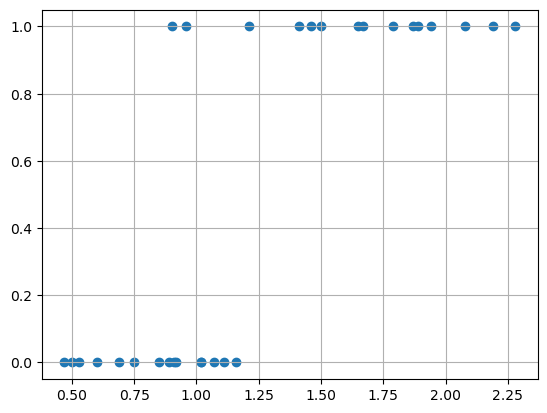
선형 회귀 분석 실시
from sklearn.linear_model import LinearRegression
from sklearn.linear_model import LogisticRegression
lr = LinearRegression()
lr.fit(X.reshape(-1, 1), y.reshape(-1, 1))
print(lr.coef_, lr.intercept_) # 기울기, 절편 출력[[0.74825276]] [-0.43007818]선형 회귀 분석 시각화
# 회귀 방정식 : y = ax + b
x = np.linspace(0.5, 2.25, 50) # 0.5~2.25 사이 간격을 50 등분 함
yy = (lr.coef_ * x) + lr.intercept_
plt.scatter(X, y, color='red')
plt.plot(x.reshape(-1,1), yy.reshape(-1,1), 'b-')
plt.grid()
plt.show()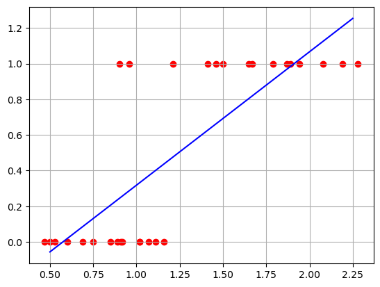
- 위 그래프에서 보듯 선형방정식은 이항분포를 따르는
데이터에 적용하기에 다소 무리가 있음- $y = ax + b$
- 즉, 우변값의 범위는 '-무한대 ~ +무한대'이지만
좌변값의 범위는 '0 ~ 1'임 - 따라서, 좌변값의 범위를 우변과 동일하게 하려면
적절한 변환함수가 필요 = > logit함수를 이용
logit함수 정의
def logistic(x, a, b):
    yy = 1 / (1 + np.exp(-(a * x + b)))
    return yy
logit 함수 변환 후 시각 화
x = np.linspace(0.5, 2.25, 50) # 0.5~2.25 사이 간격을 50 등분 함
# yy = logistic(x, lr.coef_, lr.intercept_) # 앞에서 구한 기울기와 절편은 맞지 않음
yy = logistic(x, 8, -10) # 예제에 맞는 기울기와 절편을 설정 함
plt.scatter(X, y, c=y)
plt.plot(x.reshape(-1,1), yy.reshape(-1,1), 'b-')
plt.grid()
plt.show()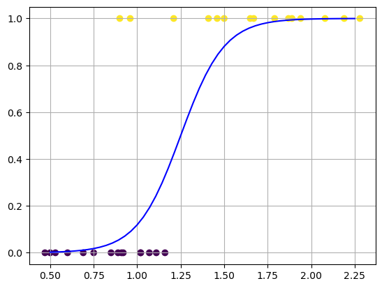
결정 경계시각화
x = np.linspace(0.5, 2.25, 50)
yy = logistic(x, 8, -10)

# yy 값이 0.5에 가장 근접한 x값을 찾음
idx = np.min(np.where(yy >= 0.5))
xp = x[idx]

plt.scatter(X, y, c=y)
plt.plot(x.reshape(-1,1), yy.reshape(-1,1), 'b-')
plt.plot([xp, xp], [-0.25, 1.25], 'r--') # 결정 경계 시각화
plt.grid()
plt.show()
# 결정계수 값
xp
1.25로지스틱 회귀로 곤충 암수 구분
pd.Series(y).value_counts()1 15
0 15
dtype: int64from sklearn.model_selection import train_test_split
X_train, X_test, y_train, y_test = train_test_split(X, y, train_size = 0.7,
stratify=y, random_state=2211171625)
lrclf = LogisticRegression()
lrclf.fit(X_train, y_train)
pred = lrclf.predict(X_test)
accuracy_score(y_test, pred)---------------------------------------------------------------------------
NameError Traceback (most recent call last)
Cell In [1], line 2
1 from sklearn.model_selection import train_test_split
----> 2 X_train, X_test, y_train, y_test = train_test_split(X, y, train_size = 0.7,
3 stratify=y, random_state=2211171625)
5 lrclf = LogisticRegression()
6 lrclf.fit(X_train, y_train)
NameError: name 'X' is not definedprecision_score(y_text, pred)recall_score(y_test, pred)결정경계 시각화
#!pip install mlxtendfrom sklearn.datasets import make_blobs
X, y = make_blobs(n_samples=100, centers=2, cluster_std=1.0, random_state=2211171645)
# make_blobs를 이용해서 정규분포를 따르는 가상데이터 생성
# n_samples : 표본수
# centers : 군집수
# cluster_std : 군집의 표준편차 (흩어짐 정도)
plt.scatter(X[:, 0], X[:, 1], c=y, s=10)
plt.show()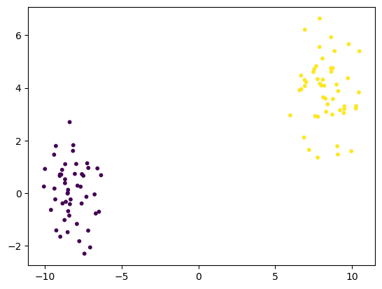
lrclf = LogisticRegression()
lrclf.fit(X, y)
lrclf.score(X, y) # 학습시 정확도
# accuracy_score(y_test, pred)1.0from mlxtend.plotting import plot_decision_regions
plot_decision_regions(X, y, clf=lrclf) # X는 2차원이어야 함
plt.show()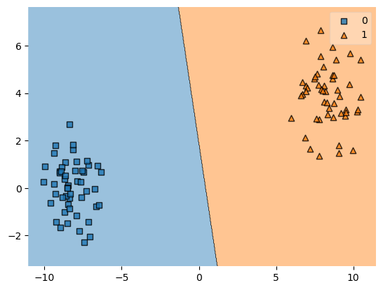
728x90
'PYTHON > 데이터분석' 카테고리의 다른 글
| [머신러닝] 10. 엔트로피 (1) | 2023.01.03 |
|---|---|
| [머신러닝] 09. 의사결정 나무 (0) | 2023.01.03 |
| [머신러닝] 07. ROC 그래프 (0) | 2023.01.03 |
| [머신러닝] 06. 오차행렬 (0) | 2023.01.03 |
| [머신러닝] 05. 데이터 전처리 (0) | 2023.01.03 |
'PYTHON/데이터분석' Related Articles
more


Comments